Dropdown lists are one of those features that seem complicated until you learn them, and then you wonder how you ever lived without them. They prevent typos, save time, keep your data consistent, and make spreadsheets actually pleasant to use. Yet somehow, most people have no idea they exist.
I’m going to show you exactly how to create dropdown lists in both Excel and Google Sheets. The process is slightly different for each, but both are surprisingly simple once you know where to click.
Why You Actually Need Dropdown Lists
Before we dive into the how, let’s talk about the why. Dropdown lists solve three massive problems:
Problem 1: The Typo Nightmare
When you’re collecting data from multiple people, someone will always misspell something. “Approved,” “aproved,” “Aprooved,” “APPROVED” – all different values to a spreadsheet, even though they mean the same thing. Dropdown lists eliminate this entirely.
Problem 2: The Speed Issue
Typing the same values repeatedly is mind-numbingly slow. Status updates, department names, product categories – if you’re entering them more than five times, you need a dropdown list.
Problem 3: The Consistency Problem
Let’s say you’re tracking projects by status: “In Progress,” “Complete,” “On Hold.” Without a dropdown, someone inevitably types “In-Progress” or “Completed” or “Waiting” instead. Now your data is a mess, and any filters or formulas you built stop working.
Dropdown lists fix all of this. One click, consistent data, zero typos.
How to Create a Dropdown List in Excel
Excel has two main methods for creating dropdown lists. I’ll show you both, starting with the easiest.
Method 1: The Quick List (For Simple Dropdowns)
Use this method when you have a short list of options that won’t change much.
Step 1: Select Your Cells
Click the cell where you want the dropdown. If you want multiple cells to have the same dropdown, select all of them at once. You can select an entire column by clicking the column letter at the top.
Step 2: Open Data Validation
Go to the Data tab in the ribbon at the top. Look for the Data Tools section, then click Data Validation. A dialog box will appear.
Step 3: Set Your Criteria
In the dialog box:
- Under “Allow,” select List from the dropdown (yes, you’re using a dropdown to create a dropdown)
- In the “Source” field, type your options separated by commas
- Example:
None, To do, In Progress, For Checking, Checked, ApproveNone; To do; In Progress; For Checking; Checked; Approved;
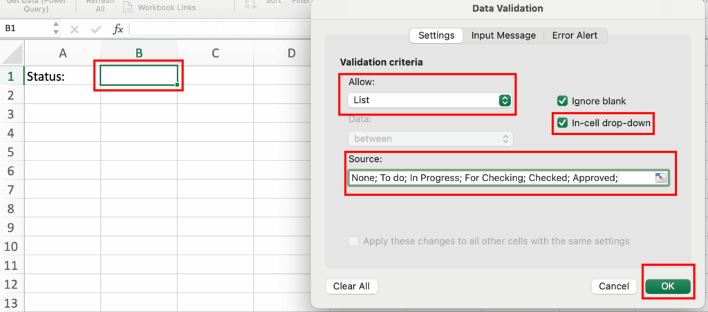
Make sure “In-cell dropdown” is checked. This is what creates that little arrow next to the cell.
Step 4: Done
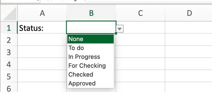
Click OK. Your dropdown is now live. Click any cell you selected, and you’ll see a small arrow appear. Click it to choose from your list.
Method 2: The Reference Method (For Longer Lists)
This is the smarter approach for longer lists or lists that might change over time.
Step 1: Create Your List Somewhere
Pick a spot on your spreadsheet (or even a different sheet) to type out your list. One item per cell, going down vertically.
For example, in cells H1 through H10, type:
- None
- To Do
- In Progress
- For Checking
- Checked
- Approved
- Rejected
- Pending
- Under Review
- Cancelled
Step 2: Select Your Dropdown Cells
Click the cells where you want the dropdown to appear. This is usually in a different column from where you just created your list.
Step 3: Open Data Validation
Data tab → Data Validation (same as Method 1).
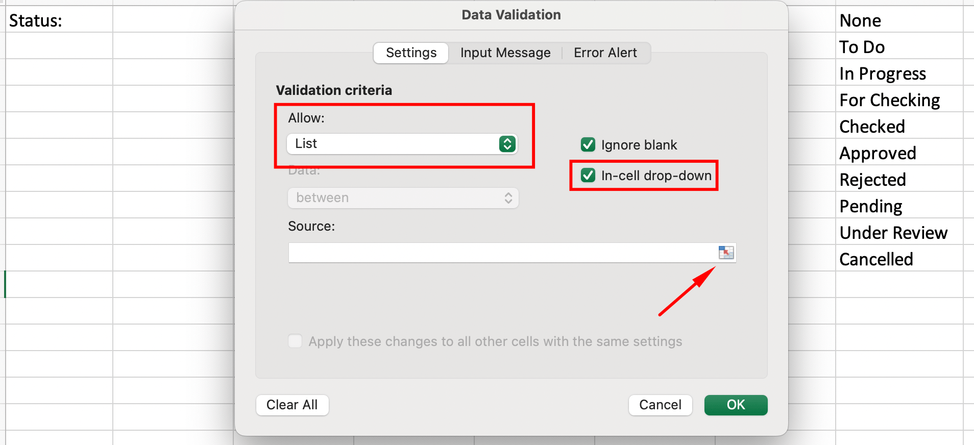
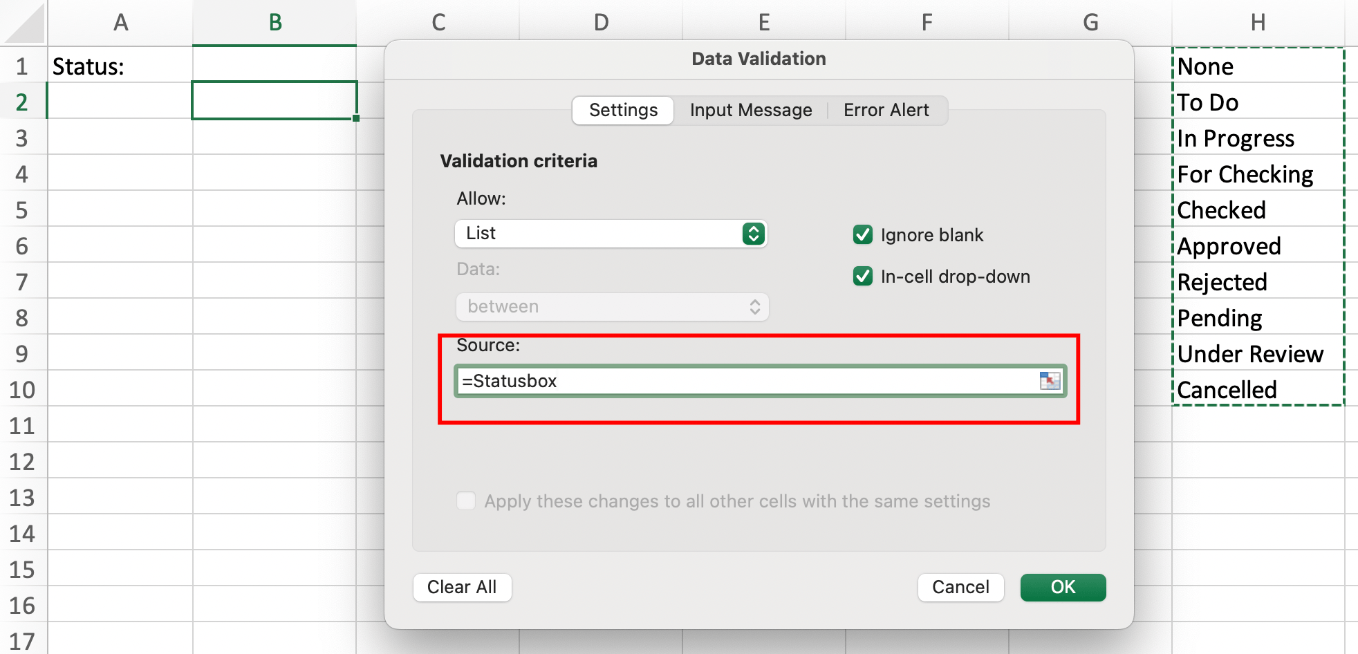
Step 4: Reference Your List
In the dialog box:
- Under “Allow,” select List
- In the “Source” field, click the little upward arrow icon (or just click in the field)
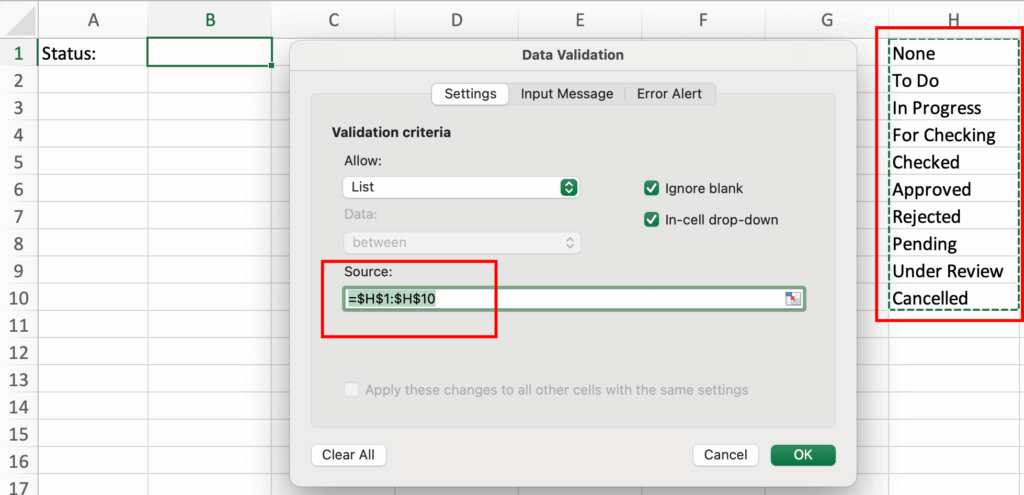
- Go select your list – click and drag from H1 to H10 (or wherever your list is)
- You’ll see something like
=$H$1:$H$10appear in the Source field - Make sure “In-cell dropdown” is checked
Step 5: Finish
Click OK. Now your dropdown pulls from that list you created. The best part? If you need to add or change options later, just edit that reference list – every dropdown updates automatically.

Pro Tips for Excel Dropdowns
Tip 1: Named Ranges Make Life Easier
Instead of remembering cell references like $H$1:$H$10, you can name that range:
- Select your list (H1:H10)
- Click in the Name Box (that’s the box at the far left, above column A, that shows the cell reference)
- Type a name like “Statusbox” (no spaces allowed)
- Press Enter
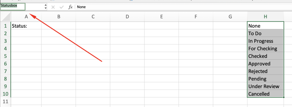
Now when you create a dropdown, just type =StatusList in the Source field. Much cleaner.
Tip 2: Create Dependent Dropdowns
This is advanced but incredibly useful. Let’s say you have a dropdown for “Department” and you want a second dropdown for “Team” that changes based on which department is selected.
Here’s the quick version:
- Create separate lists for each department’s teams
- Name each list (SalesTeams, MarketingTeams, etc.)
- In the second dropdown’s Data Validation, use an INDIRECT formula:
=INDIRECT(A2)where A2 is the cell with the first dropdown - Make sure your list names match exactly what’s in the first dropdown
It’s tricky the first time, but once you get it working, it’s magical.
Tip 3: Show an Input Message
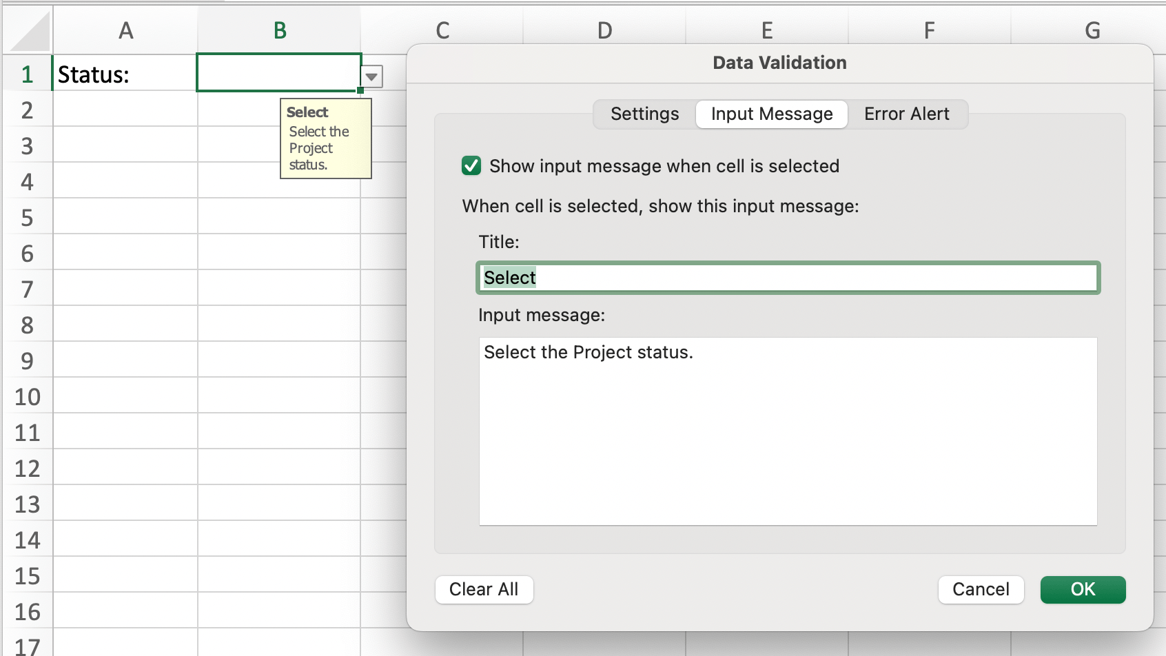
In the Data Validation dialog, click the “Input Message” tab. You can add a title and message that appears when someone selects the cell. Use it for instructions like “Select project status from the list.”
Tip 4: Set Up Error Alerts
Also in Data Validation, the “Error Alert” tab lets you customize what happens if someone tries to type something that’s not in your list. You can show a warning or completely block invalid entries.
How to Create a Dropdown List in Google Sheets
Google Sheets handles dropdowns differently from Excel – actually, I think their method is cleaner. Here’s how it works.
Method 1: Quick List from Scratch
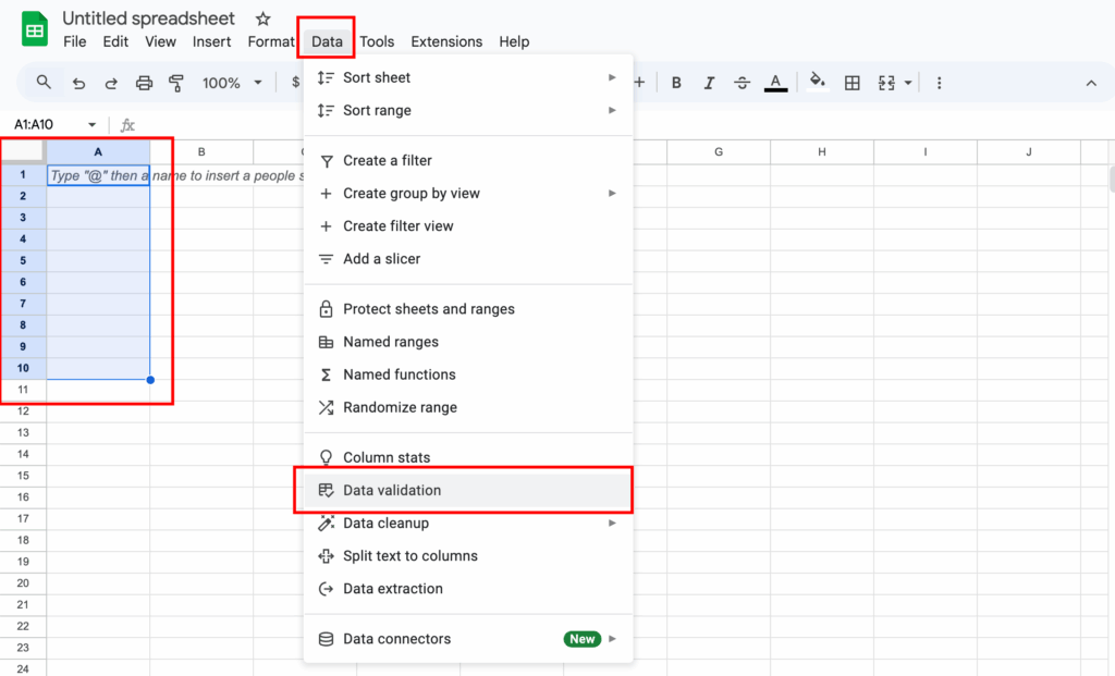
Step 1: Select Your Cell(s)
Click the cell where you want the dropdown. To apply it to multiple cells, select the entire range at once.
Step 2: Open Data Validation
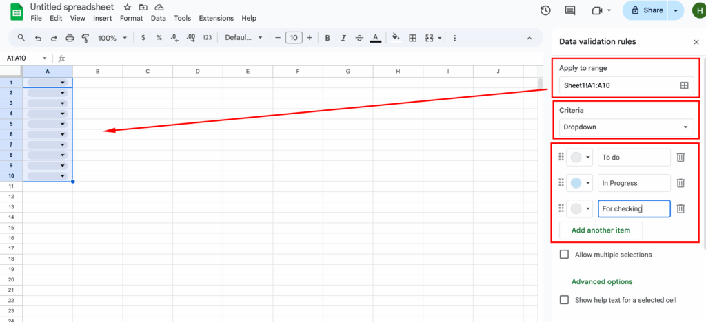
Click Data in the menu bar, then choose Data validation. A panel will open on the right side of your screen.
Step 3: Set Up Your List
In the data validation panel:
- Make sure “Cell range” shows the cells you selected
- Under “Criteria,” choose Dropdown (from a range) or Dropdown
- If you chose “Dropdown,” a text box appears where you type your options
- Type each option and press Enter after each one
- Example:
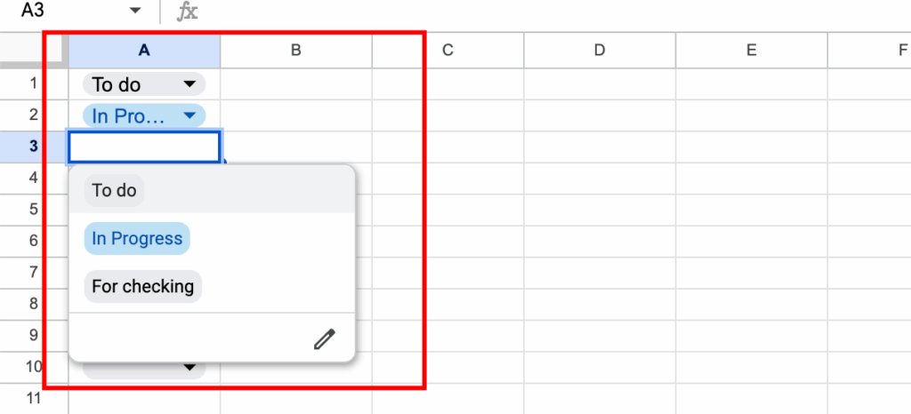
- To Do
- In Progress
- For Checking
Step 4: Choose Display Options
You’ll see options for:
- Show dropdown list in cell: Keep this checked (that’s the whole point)
- Show validation help text: Optional – adds a note visible when the cell is selected
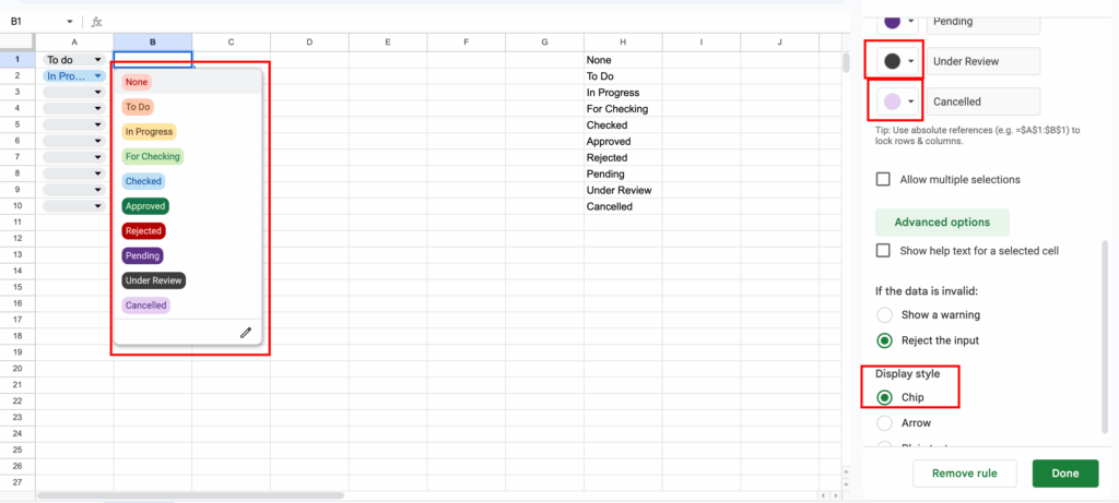
- Appearance: Choose whether to show the list as chips (colorful tags) or plain text
Step 5: Set Rejection Rules
Under “On invalid data”:
- Show warning: Allows invalid entries but shows a warning
- Reject input: Blocks anything not on your list (recommended)
Step 6: Save
Click Done. Your dropdown is ready.
Method 2: Dropdown from a Range
This is similar to Excel’s reference method and better for longer lists.
Step 1: Create Your Source List
Somewhere on your sheet (I usually use a column far to the right or a separate tab), type your list vertically, one item per cell.
Step 2: Select Target Cells
Click the cells where you want dropdowns to appear.
Step 3: Open Data Validation
Data → Data validation (same as before).
Step 4: Choose Range
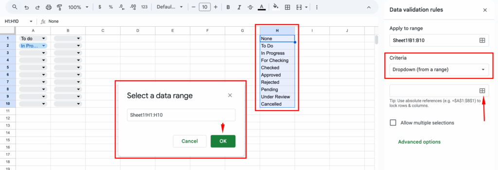
Under “Criteria,” select Dropdown (from a range).
A field appears asking for the range. Click the grid icon, then select your source list. You’ll see something like Sheet1!H1:H10 appear.
Step 5: Configure and Save
Set your display options and rejection rules, then click Done.

Now when you update your source list, all dropdowns update automatically.
Google Sheets Advanced Features
Feature 1: Color-Coded Dropdown Chips
In the data validation panel, under “Appearance,” select Chip. Then click “Customize chip color” to assign different colors to different options. This makes status dropdowns incredibly visual.
Feature 2: Multi-Select Dropdowns
Google Sheets can do something Excel can’t (at least not easily): allow users to select multiple items from one dropdown.
When setting up data validation, look for the checkbox “Allow multiple selections in the same cell.” Enable it, and users can select multiple options, which appear as separate chips in the cell.
Feature 3: Criteria Formulas
Under “Criteria,” you can also choose “Custom formula is” and write a formula to determine valid entries. This is powerful for complex validation rules.
Example: Only allow dates in the future =A2>TODAY()
Example: Only allow numbers between 1 and 100 =AND(A2>=1, A2<=100)
Common Mistakes to Avoid
Mistake 1: Not Protecting Your Source List
If your dropdown references a list and someone accidentally deletes that list, all your dropdowns break. Either:
- Put source lists on a hidden sheet
- Lock the cells containing source lists
- Use a separate “Data” sheet that regular users don’t access
Mistake 2: Including Blank Cells in Your Range
If your source list is H1:H10 but only H1:H6 have values, your dropdown will show four blank options. Either:
- Use only the filled cells (H1:H6)
- Or type something in the blank cells like “N/A” or delete the blank rows
Mistake 3: Forgetting to Apply to the Whole Column
You create a perfect dropdown for cell B2, then forget to apply it to B3:B100. Weeks later, someone types random values in B45, and your data is inconsistent again. Always select the entire range you need upfront.
Mistake 4: Making Lists Too Long
Dropdowns with 50+ items become unusable. If your list is that long, consider:
- Breaking it into multiple dependent dropdowns
- Using search functionality instead
- Grouping items into categories first
Quick Comparison: Excel vs Google Sheets
| Feature | Excel | Google Sheets |
|---|---|---|
| Setup complexity | Slightly more steps | Cleaner interface |
| Color-coded options | Requires conditional formatting | Built-in chip colors |
| Multi-select | Requires VBA or workarounds | Native support |
| Dependent dropdowns | Need INDIRECT formula | Need INDIRECT formula |
| Offline access | Always available | Requires setup |
| Collaboration | Can be tricky | Seamless |
Neither is “better” – it depends on your needs. I use Excel for complex financial models and Google Sheets for team collaboration.
Real-World Use Cases
Use Case 1: Project Management
Columns for Status, Priority, and Assigned To, all with dropdowns. No more “in progress” vs “In Progress” vs “In-Progress” chaos.
Use Case 2: Expense Tracking
Category dropdown (Travel, Meals, Office Supplies, etc.) ensures consistent categorization for accounting and analysis.
Use Case 3: Customer Database
Dropdowns for Industry, Lead Source, Deal Stage, and Region. Makes filtering and reporting actually work.
Use Case 4: Inventory Management
Location dropdown ensures products are tracked to actual warehouse zones, not “Zone A” vs “A Zone” vs “Area A.”
Use Case 5: Surveys and Forms
Yes/No questions, rating scales, multiple choice – all perfect for dropdowns.
Troubleshooting Common Issues
Problem: Dropdown arrow doesn’t appear
Solution: Go back to Data Validation and make sure “In-cell dropdown” (Excel) or “Show dropdown list in cell” (Google Sheets) is checked.
Problem: Getting an error message when selecting from dropdown
Solution: Your source range might include empty cells or invalid data. Check your source list and ensure it only contains the values you want.
Problem: Dropdown shows numbers instead of text
Solution: Your source cells might be formatted as numbers. Change them to text format, or add an apostrophe before each entry (‘1, ‘2, ‘3) to force text.
Problem: Can’t select multiple items (Google Sheets)
Solution: In Data validation, you need to specifically enable “Allow multiple selections in the same cell.” It’s not on by default.
Problem: Dropdown disappeared after sorting
Solution: Your data validation is still there, but if you sorted a range that included cells without validation, the rules don’t move with the data. You’ll need to reapply validation to the new cell positions.
The Bottom Line
Dropdown lists are one of those features that seem unnecessary until you use them, and then you can’t imagine working without them. They take literally two minutes to set up and save hours of fixing typos and inconsistent data.
Start simple. Pick one spreadsheet you use regularly and add dropdowns to just one column. Once you see how much cleaner your data becomes, you’ll start adding them everywhere.
And next time someone is manually typing the same six values into 200 cells, you can be the hero who shows them the better way.
